Data access using the low-level API#
This guide demonstrates how to access raw data using aeon_api, Aeon’s low-level API. In this example, we are using the Single Mouse Foraging Assay – 2-Hour Sample dataset.
Set up environment#
To get started, install the aeon_mecha package from the aeon_docs branch by following the steps in the installation guide.
This will automatically install aeon_api and all other required dependencies.
You can also run this notebook online at works.datajoint.com using the following credentials:
Username: aeondemo
Password: aeon_djworks
To access it, go to the Notebook tab at the top and in the File Browser on the left, navigate to ucl-swc_aeon > docs > examples, where this notebook io_api_example.ipynb is located.
Import libraries#
from dataclasses import asdict
from typing import cast

import pandas as pd
import swc
from matplotlib import pyplot as plt
from swc.aeon.analysis.plotting import heatmap
from swc.aeon.analysis.utils import distancetravelled
from swc.aeon.io.video import frames

from aeon.metadata.social_02 import ExperimentMetadata
from aeon.schema.schemas import social02
The root path is the directory containing the entire dataset, including all epochs and chunks of data for all streams of all devices. If your local dataset is in a different location, please change the value below before running the cells below.
root = "/data/raw/AEON3/social0.2/"
# If you are running this notebook on `works.datajoint.com`, use the following path instead:
# root = "/home/jovyan/inbox/aeon/data/raw/AEON3/social0.2/"
Experiment metadata#
Information about the location and configuration of all devices can be extracted from the Metadata.yml file. The ExperimentMetadata class provides a convenient API for parsing and accessing this metadata to access video frame rate, pixel to standard unit conversions, etc.
metadata = swc.aeon.load(root, social02.Metadata)["metadata"].iloc[0]
experiment = ExperimentMetadata(metadata)
arena = experiment.arena
asdict(experiment)
{'arena': {'radius_cm': 100.0,
  'radius_px': 531.0,
  'center_px': array([708., 543.]),
  'pixel_to_cm': 0.18832391713747645},
 'video': {'global_fps': 50.0, 'local_fps': 125.0},
 'patch1': {'radius_cm': -4.0,
  'roi_px': array([[899., 535.],
         [922., 533.],
         [921., 554.],
         [899., 554.]])},
 'patch2': {'radius_cm': -4.0,
  'roi_px': array([[610., 709.],
         [628., 718.],
         [617., 739.],
         [600., 730.]])},
 'patch3': {'radius_cm': -4.0,
  'roi_px': array([[590., 371.],
         [608., 360.],
         [619., 380.],
         [601., 392.]])},
 'nest': {'roi_px': array([[1321.,  486.],
         [1231.,  485.],
         [1231.,  591.],
         [1323.,  583.]])},
 'patch1_rfid': {'location_px': array([940., 542.])},
 'patch2_rfid': {'location_px': array([600., 753.])},
 'patch3_rfid': {'location_px': array([589., 348.])},
 'nest_rfid1': {'location_px': array([1218.,  642.])},
 'nest_rfid2': {'location_px': array([1214.,  426.])},
 'gate_rfid': {'location_px': array([195., 563.])}}
Position tracking#
The social02 schema is used with the aeon.load function to read stream data from different devices. Below we access the SLEAP pose data from CameraTop and convert pixel coordinates to standard units using the point_to_cm function from arena metadata.
pose = swc.aeon.load(root, social02.CameraTop.Pose)
position_cm = experiment.arena.point_to_cm(pose[["x", "y"]])
In single-subject datasets, the pose DataFrame holds data for one animal.
In multi-animal datasets, it includes pose data for several mice, with each one’s identity labelled.
pose
| identity | identity_likelihood | part | x | y | part_likelihood | |
|---|---|---|---|---|---|---|
| time | ||||||
| 2024-03-02 12:00:00.039999962 | BAA-1104047 | 0.972604 | anchor_centroid | 1306.963623 | 496.801605 | 0.932558 |
| 2024-03-02 12:00:00.039999962 | BAA-1104047 | 0.972604 | centroid | 1306.547363 | 496.642487 | 0.924312 |
| 2024-03-02 12:00:00.099999905 | BAA-1104047 | 0.963363 | anchor_centroid | 1306.954468 | 496.790466 | 0.934447 |
| 2024-03-02 12:00:00.099999905 | BAA-1104047 | 0.963363 | centroid | 1306.537598 | 496.609711 | 0.923661 |
| 2024-03-02 12:00:00.159999847 | BAA-1104047 | 0.959149 | anchor_centroid | 1306.940063 | 496.785583 | 0.938 |
| ... | ... | ... | ... | ... | ... | ... |
| 2024-03-02 13:59:59.860000134 | BAA-1104047 | 0.739153 | centroid | 1304.156006 | 579.062988 | 0.946275 |
| 2024-03-02 13:59:59.920000076 | BAA-1104047 | 0.713065 | anchor_centroid | 1304.555908 | 579.327637 | 0.945027 |
| 2024-03-02 13:59:59.920000076 | BAA-1104047 | 0.713065 | centroid | 1304.1698 | 579.047119 | 0.948602 |
| 2024-03-02 13:59:59.980000019 | BAA-1104047 | 0.702433 | anchor_centroid | 1304.551025 | 579.312561 | 0.946382 |
| 2024-03-02 13:59:59.980000019 | BAA-1104047 | 0.702433 | centroid | 1304.168945 | 579.033264 | 0.945419 |
239990 rows × 6 columns
position_cm
| x | y | |
|---|---|---|
| time | ||
| 2024-03-02 12:00:00.039999962 | 112.799176 | -8.700263 |
| 2024-03-02 12:00:00.039999962 | 112.720784 | -8.730229 |
| 2024-03-02 12:00:00.099999905 | 112.797452 | -8.70236 |
| 2024-03-02 12:00:00.099999905 | 112.718945 | -8.736401 |
| 2024-03-02 12:00:00.159999847 | 112.794739 | -8.70328 |
| ... | ... | ... |
| 2024-03-02 13:59:59.860000134 | 112.270434 | 6.791523 |
| 2024-03-02 13:59:59.920000076 | 112.345745 | 6.841363 |
| 2024-03-02 13:59:59.920000076 | 112.273032 | 6.788535 |
| 2024-03-02 13:59:59.980000019 | 112.344826 | 6.838524 |
| 2024-03-02 13:59:59.980000019 | 112.272871 | 6.785925 |
239990 rows × 2 columns
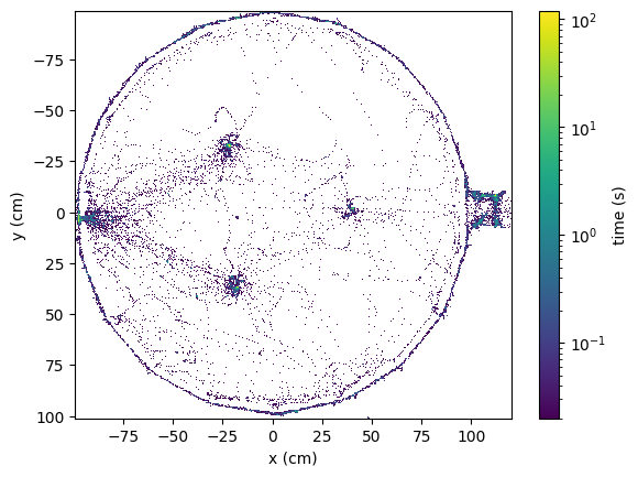
The low-level API also contains utility functions for data visualisation and exploration.
Below we use the heatmap function to display a 2D histogram of the position data over the entire dataset period.
fig, ax = plt.subplots(1, 1)
heatmap(position_cm, experiment.video.global_fps, bins=500, ax=ax)
ax.set_xlabel("x (cm)")
ax.set_ylabel("y (cm)")
plt.show()
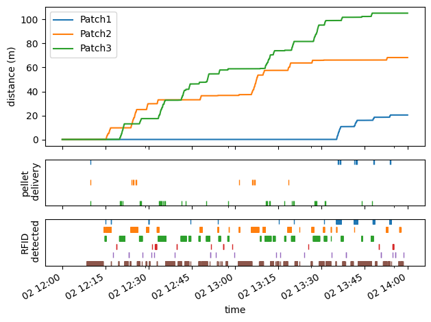
Foraging activity#
In this experiment there are three foraging patches. For each patch we access below the wheel movement data and state transitions when a pellet is delivered.
patches = ["Patch1", "Patch2", "Patch3"]
patch_encoder = {patch: swc.aeon.load(root, social02[patch].Encoder) for patch in patches}
patch_distance = {
    patch: distancetravelled(patch_encoder[patch].angle, radius=experiment.patch1.radius_cm / 100)
    for patch in patches
}
pellet_deliveries = {
    patch: swc.aeon.load(root, social02[patch].DepletionState)
    .groupby(pd.Grouper(freq="1s"))
    .first()
    .dropna()
    for patch in patches
}
RFID tag readers are also located at various points of the environment and can be accessed using the same API.
rfids = ["Patch1Rfid", "Patch2Rfid", "Patch3Rfid", "NestRfid1", "NestRfid2", "GateRfid"]
rfid_events = {rfid: swc.aeon.load(root, social02[rfid].RfidEvents) for rfid in rfids}
Below we summarise all patch and RFID activity.
Tip
Since data is synchronised at source, we can directly align time across all plots.
fig, axes = plt.subplots(3, 1, sharex=True, height_ratios=[0.6, 0.2, 0.2])

for i, patch in enumerate(patches):
    # plot distance travelled and pellet delivery events
    patch_distance[patch].plot(ax=axes[0], label=patch, x_compat=True)
    pellet_deliveries[patch].assign(patch_index=-i).patch_index.plot(ax=axes[1], style="|", label=patch)

for i, rfid in enumerate(rfids):
    # plot RFID detection events
    rfid_events[rfid].assign(rfid_index=-i).rfid_index.plot(ax=axes[2], style="|", label=rfid)

axes[0].set_ylabel("distance (m)")
axes[1].set_ylabel("pellet\n delivery")
axes[2].set_ylabel("RFID\n detected")
axes[1].set_yticks([])
axes[2].set_yticks([])
axes[0].legend()
plt.tight_layout()
plt.show()
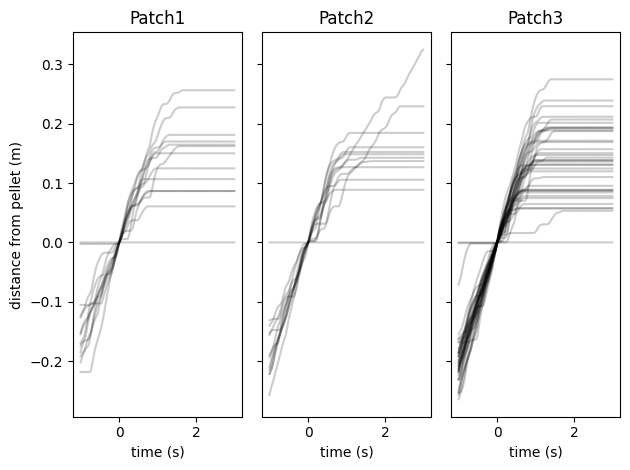
Event-triggered analysis#
Having the same time reference for all data is also useful for quick exploration of correlations. Below we correlate wheel movement data with pellet delivery events by performing a direct outer join between the two tables and grouping by event count.
fig, axes = plt.subplots(1, 3, sharey=True)

for i, patch in enumerate(patches):
    # get patch state at each pellet delivery
    patch_state = pellet_deliveries[patch].assign(count=pellet_deliveries[patch].offset.notna().cumsum())

    # correlate patch state with wheel data with a time delay
    foraging_state = patch_state.shift(freq="-1s").join(patch_distance[patch], how="outer").ffill().dropna()

    # group wheel data by pellet delivery and align on first second
    for _, v in foraging_state.groupby("count"):
        foraging_distance = v.head(200).distance.to_frame()
        foraging_distance -= foraging_distance.iloc[50]
        foraging_distance.index = (foraging_distance.index - foraging_distance.index[50]).total_seconds()
        foraging_distance.distance.plot(ax=axes[i], style="k", alpha=0.2)
    axes[i].set_title(patch)
    axes[i].set_ylabel("distance from pellet (m)")
    axes[i].set_xlabel("time (s)")

plt.tight_layout()
plt.show()
Video analysis#
The aeon.io.video module includes utilities for easily extracting raw video frames and movies aligned to the data.
camera_frames = {
    "CameraTop": swc.aeon.load(root, social02.CameraTop.Video),
    "CameraPatch1": swc.aeon.load(root, social02.CameraPatch1.Video),
    "CameraPatch2": swc.aeon.load(root, social02.CameraPatch2.Video),
    "CameraPatch3": swc.aeon.load(root, social02.CameraPatch3.Video),
    "CameraNest": swc.aeon.load(root, social02.CameraNest.Video),
}
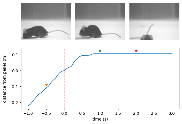
Below we extract the normalised wheel distance before and after a single pellet delivery on a specified patch. As above we normalise time in seconds aligned to pellet delivery and distance in meters from pellet.
single_patch = "Patch2"
delivery_index = 6
before_delta = pd.Timedelta("1s")
after_delta = pd.Timedelta("3s")

single_pellet = pellet_deliveries[single_patch].iloc[delivery_index]
delivery_time = cast(pd.Timedelta, single_pellet.name)
before = delivery_time - before_delta
after = delivery_time + after_delta
foraging_distance = (
    patch_distance[single_patch].loc[before:after] - patch_distance[single_patch].loc[delivery_time]
)
foraging_distance.index = (foraging_distance.index - delivery_time).total_seconds()
Next we extract the video frames corresponding to specific moments in the pellet delivery sequence.
Note how reindex is used with ffill to get the closest frame following the desired frame times.
Given a DataFrame of video frame metadata, the frames function will open and decode all the corresponding frame data as a numpy.array.
# get video frames at specific offsets from delivery time
frame_deltas_seconds = [-0.5, 1, 2]
frame_times = [delivery_time + pd.Timedelta(delta, unit="s") for delta in frame_deltas_seconds]
frame_metadata = camera_frames[f"Camera{single_patch}"].reindex(frame_times, method="ffill")
bout_frames = list(frames(frame_metadata))
Finally we arrange a mosaic plot drawing each individual frame from left to right and annotate the distance plot with the frame times.
fig, axes = plt.subplot_mosaic([["A", "B", "C"], ["D", "D", "D"]])
foraging_distance.plot(ax=axes["D"])
for i, frame_delta in enumerate(frame_deltas_seconds):
    ax_index = chr(ord("A") + i)
    axes[ax_index].imshow(bout_frames[i])
    axes[ax_index].set_axis_off()
    axes["D"].plot(frame_delta, foraging_distance.loc[frame_delta] + 0.02, "*")
axes["D"].axvline(0, linestyle="--", color="red")
axes["D"].set_ylabel("distance from pellet (m)")
axes["D"].set_xlabel("time (s)")
plt.tight_layout()
plt.show()